This activity is about image segmentation, as the title suggests :). In this activity, we were tasked to isolate a portion or portions of an image. We call this our region of interest (ROI), and all other portions as the background.
Before we go to the activity proper, we first discuss an important concept -- normalized chromaticity coordinates (discussion is based on the activity sheet prepared by ma'am Soriano). With RGB values, things are quite complex since we need 3 values: R, G, and B. To simplify things, we shift to the normalized chromaticity space where we only need 2 values to describe color. Using the RGB values, we compute for a total intensity for each pixel \( I = R + G + B \). Then, we calculate for the normalized chromaticity coordinates \( r,g,b \)
$$r = \dfrac{R}{I}$$
$$g = \dfrac{G}{I}$$
$$b = \dfrac{B}{I}$$
Note that since the RGB values are normalized with respect to their sum, the sum of the normalized coordinates is 1, and so we have \( r + g + b = 1 \). Using this, we see that we now only need 2 values to describe color since the 3rd value is dependent on the other 2 (say \( b = 1 - r - g \), so we only need \( r,g \) values). Plotted below is a visualization of the colors in the normalized chromaticity space.
 |
| Normalized chromaticity space Image from https://upload.wikimedia.org/wikipedia/en/thumb/7/7b/Rg_normalized_color_coordinates.png/800px-Rg_normalized_color_coordinates.png |
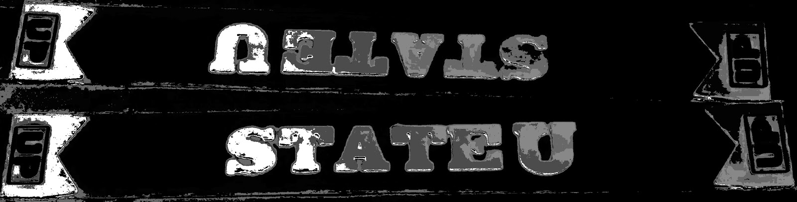
Now we go to segmenting an image! First, we need an image with portions that have a single color only. So I looked inside my bag for something I could use, and I saw my ID lace. So I took a photo, and cropped the important portion I need. The image is shown below.
 |
| Image subject for segmentation |
We focus first on using a parametric probability distribution. Basically, we assume here a Gaussian probability distribution (based on a color patch) that a color is part of our ROI. We have a probability distribution \( p(r) \) that coordinate \(r\) in the image is in our ROI, and probability distribution \(p(g)\) that coordinate \(g\) in the image is in our ROI. These are given by
$$p(r) = \dfrac{1}{\sigma_r \sqrt{2\pi}} \exp{\left[ \dfrac{-(r - \mu_r)^2}{2\sigma_{r}^2} \right]}$$
$$p(g) = \dfrac{1}{\sigma_g \sqrt{2\pi}} \exp{\left[ \dfrac{-(g - \mu_g)^2}{2\sigma_{g}^2} \right]}$$
where \( \mu_r , \mu_g \) are the means of \( r,g \) in the color patch, and \( \sigma_r,\sigma_g \) are the standard deviations of \( r,g \) in the color patch. We then have a joint probability by multiplying the 2 probability distributions \( p(r) p(g) \). With the values of the joint probabilty, we can already visualize our segmented image by using these as the values of our image array (rescale the values to a range of 0-255). The resulting image is shown below.
 |
| Segmented image using the raw values of the joint probabilities |
Considering only the raw values of the joint probabilities as the intensities of the pixels does not produce a good segmentation of our ROI. One thing we can do is set a threshold value for the joint probability, where if the values are greater than this threshold, we consider it as part of our ROI, and if the values are less than the threshold, these are not part of the ROI. The results of the image segmentation using different set threshold values are shown below.


Segmented images using a parametric probability distribution with decreasing threshold values of the joint probability from top to bottom (10-6,10-12,10-18,10-24,10-30)
Note that as the threshold is decreased, the ROI is completed, obtaining more and more information towards the right. This can be explained by the non-uniform illumination of the subject. In the original image, the illumination is greater in the righthand portion of the image. This non-uniform illumination causes changes in the values of RGB, and consequently \(rg\). So, the values deviate farther from the mean, and causes a decrease in probability.
Next, we use non-parametric probability distribution in segmenting our image. In this method, we use the histogram of the color patch (in \( rg \) space) itself as our probability distribution. What we do is to take note of the \(r,g\) value of each pixel in the image, refer to the value of the point (\(r,g\)) in the histogram, and use this as the value of the pixel in the image. This is called histogram backprojection. (Again, this discussion is based on the activity sheet prepared by ma'am Soriano :) )
Now we go on to segmenting our image. First we get the histogram of our image. A code was provided in the activity sheet to implement this; I tried it but it would not run, and I could not debug it because I couldn't quite understand the flow of the code. So, I made a code to implement the histogram creation, along with the backprojection portion of the process (the code is included below, including the code used to implement image segmentation using parametric probability distribution). The histogram of the color patch is shown below.
 |
| Color histogram of the color patch |
 |
| Segmented image using non-parametric probability distribution |
Of course, we can also use a threshold value as done earlier. If we again set a threshold value and decrease it, we will again see a more and more distinct segmentation. But, instead of doing this, I thought of using another color patch in addition to the 1st color patch, so as to add more counts in the color histogram. So, I took a color patch from the ROI in the right. The updated histogram and the segmented image is shown below.
 |
| Updated color histogram using the 2 color patches |
 |
| Segmented image using non-parametric distribution of 2 color patches |
We see that we segment more of our ROI compared to the earlier result. The use of an additional color patch enabled us to have information on the color of the right portion of the image, thus, we are also able to segment this portion of the image.
If we compare the results of the parametric and non-parametric segmentation, we see a more segmented image for the non-parametric segmentation (when considering the raw values). Of course we can improve these by setting thresholds and by adding more color patches. However, non-parametric segmentation offers a better approach since we are not assuming anything. In this process, we are using the distribution of the colors in the image itself and not assuming a certain profile distribution. The downside of assuming a profile is that it may not be fit. The fitting part already introduces errors, and so the results deviate from what we want.
I have learned so much in this activity, and I am excited about the next activities about color, and image processing. Having gone through this, I have realized that I can see myself doing things like this in the future (although I know this is still very basic. aaaand, I'm still at the crossroad, deciding what to do and what field to go to, if ever). I would give myself a grade of 11. I have done the tasks in the activity sheet, and have contributed an alternative code in implementing the histogram production. Hopefully the things I have done are enough for that kind of grade.
The code that I used for this activity are included below for reference.
1 2 3 4 5 6 7 8 9 10 11 12 13 14 15 16 17 18 19 20 21 22 23 24 25 26 27 28 29 30 31 32 33 34 35 36 37 38 39 40 41 42 43 44 45 46 47 48 49 50 51 52 53 54 55 56 57 58 59 60 61 62 63 64 65 66 67 68 69 70 71 72 73 74 75 76 77 78 79 80 81 82 83 84 85 86 | // Image img = double(imread('C:\Users\toshiba\Google Drive\College\5th year\App Physics 186\Act7\ID_edited2.jpg')); R = img(:,:,1); G = img(:,:,2); B = img(:,:,3); I = R + G + B; // Color patch ROI_color = double(imread('C:\Users\toshiba\Google Drive\College\5th year\App Physics 186\Act7\ROI-color.jpg')); R_ROI = ROI_color(:,:,1); G_ROI = ROI_color(:,:,2); B_ROI = ROI_color(:,:,3); I_ROI = R_ROI + G_ROI + B_ROI; //// Additional color patch //ROI_color2 = double(imread('C:\Users\toshiba\Google Drive\College\5th year\App Physics 186\Act7\ROI-color2.jpg')); //R_ROI2 = ROI_color2(:,:,1); G_ROI2 = ROI_color2(:,:,2); B_ROI2 = ROI_color2(:,:,3); //I_ROI2 = R_ROI2 + G_ROI2 + B_ROI2; //// Parametric probability distribution estimation r = R ./ I; g = G ./ I; r_ROI = R_ROI ./ I_ROI; g_ROI = G_ROI ./ I_ROI; rmean = mean(r_ROI); gmean = mean(g_ROI); rstdev = stdev(r_ROI); gstdev = stdev(g_ROI); N = length(r_ROI); // Probability that pixel in image with chromaticity r belongs to ROI p_r = (1. /(rstdev * sqrt(2*%pi))) * exp(-((r-rmean).^2) / (2 * rstdev^2)) * (1. / N); // Probability that pixel in image with chromaticity g belongs to ROI p_g = (1. /(rstdev * sqrt(2*%pi))) * exp(-((g-gmean).^2) / (2 * gstdev^2)) * (1. / N); // Joint probability jp = p_r .* p_g; img_seg = uint8(255*(jp/max(jp))); //img_seg = jp > 1e-30; imshow(img_seg); imwrite(img_seg, 'C:\Users\toshiba\Google Drive\College\5th year\App Physics 186\Act7\ID_param.jpg'); //// Non-parametric probability distribution estimation // Creation of 2D histogram I_ROI(find(I_ROI==0)) = 100000; r_ROI = R_ROI ./ I_ROI; g_ROI = G_ROI ./ I_ROI; bins = 32; rint = round(r_ROI * (bins-1) + 1); gint = round(g_ROI * (bins-1) + 1); hist = zeros(bins,bins); for row = 1:bins for col = 1:row hist(row,col) = length(find(gint==bins-row+1 & rint==col)); disp(string(row) + ',' + string(col)); end end // Uncomment when using additional color patch //I_ROI2(find(I_ROI2==0)) = 100000; //r_ROI2 = R_ROI2 ./ I_ROI2; g_ROI2 = G_ROI2 ./ I_ROI2; //rint2 = round(r_ROI2 * (bins-1) + 1); gint2 = round(g_ROI2 * (bins-1) + 1); //for row = 1:bins // for col = 1:row // hist(row,col) = length(find(gint==bins-row+1 & rint==col)); // disp(string(row) + ',' + string(col)); // end //end imshow(uint8(255*(hist/max(hist)))); imwrite(uint8(255*(hist/max(hist))), 'C:\Users\toshiba\Google Drive\College\5th year\App Physics 186\Act7\ID-nonparam-hist.jpg'); [rr,cc] = find(hist~=0); //indices rr2 = bins - rr + 1; // change to color value I(find(I==0)) = 100000; img(:,:,1) = img(:,:,1) ./ I; img(:,:,2) = img(:,:,2) ./ I; img(:,:,1) = round(img(:,:,1) * (bins-1) + 1); img(:,:,2) = round(img(:,:,2) * (bins-1) + 1); segmented = zeros(size(img,1), size(img,2)); for z = 1:length(rr) [a,b,c] = find(img(:,:,1) == cc(z)); for x = 1:length(a) if img(a(x), b(x), 2) == rr2(z) then segmented(a(x), b(x)) = hist(rr(z),cc(z)); end end end segmented = uint8(255*(segmented/max(segmented))); imshow(segmented); imwrite(segmented, 'C:\Users\toshiba\Google Drive\College\5th year\App Physics 186\Act7\ID-nonparam.jpg'); |