Activity 11 - Basic Video Processing

Last activity for AP 186!

Activity 10 is about video processing. Video processing is not really that different from image processing, since a video is basically a series of images. And so, what we can do is process each image that comprises the video. 

The task at hand was to experimentally determine a kinematic constant, such as the acceleration due to gravity \( g \), by processing a video capturing a kinematic event. One way to determine \( g \) was simply to drop an object from a certain height and determine the time for it to travel a certain distance. \( g \) can then be calculated using the equation

$$ g = \dfrac{2 (h_o - h)}{t^2} $$

where \(h_o\) is the initial height, \( h \) is the final height, and \(t\) is the time to reach \(h\) from \(h_o\).

The video below shows my trial in performing this activity. I dropped a red cube and captured the event using my phone. The ruler was meant to serve as reference for distance. 

The video was then converted to images using Video to JPG Converter. The series of images during the drop are shown below

To identify the object, we perform color image segmentation like we performed in one of the previous activities. I obtained the color patch of the ROI from the cube in the 1st image. However, I encountered a problem. The object is identified until the 2nd image only. Starting from the 3rd image, since the object is blurred due to its motion, it cannot be identified using the ROI used. 

Luckily, Harold offered to let me use his video (thanks Harold!) of a simple pendulum. The video is shown below. \( g \) may be calculated by knowing the period of its oscillation \(T\) and using the formula 

$$g = \dfrac{4 \pi^2 L }{T}$$

where \(L\) is the length of the string

The same thing was done, where color segmentation was performed to identify the ball. Some of the images comprising the video are shown below.

Activity 10 - Enhancement by Histogram Manipulation

The sem's almost over! One more activity after this and I'm done with blogging for AP 186. One more activity after this and then AP 186 exam. Although, an exemption from taking the final exam is possible, and I do hope I qualify.

On to the activity! Activity 10 is about enhancement of  features in an image by manipulation of its histogram. Take for example a grayscale image. First, we take the probability distribution function (PDF) of the grayscale intensities, by taking the histogram of the grayscale intensities and normalizing it by the total number of pixels. We then take the cumulative distribution function (CDF) from the PDF (refer to the link for CDF information https://onlinecourses.science.psu.edu/stat414/node/98). To manipulate the histogram, we backproject the grayscale intensities with a desired CDF of ours. Following the discussion in out manual (thank you ma'am Jing), if we for example have \( A(x) \) as the CDF of our image, and \( B(y) \) is our desired CDF, then for each pixel intensity in out image, we transform it to \( y = B^{-1}(A(x)) \). In other words, if we have a pixel intensity \(x\), we determine its corresponding CDF value \( A(x) \), then determine the corresponding \(y\) value that produces \( B(y) = A(x) \).

Let's take for example the image shown below. We first convert this image to grayscale, which is also shown below. 

Image A

Image A in grayscale

We then manipulate the histogram of this image. The PDF and CDF of this image is shown below. We backproject this CDF using a linear CDF, which runs from (0,0) to (255,1). This equalizes the histogram of the image. The resulting image is shown below. 

PDF of image A in grayscale

CDF of image A in grayscale

Grayscale image A after histogram equalization

The colored image can also be enhanced by histogram manipulation. If we convert the \(RGB\) values to \(rgI\) values, histogram manipulation can be done on the \( I \) values. The \(I\) values were normalized with respect to the maximum value \(I_{max}\), then the histogram was obtained. The PDF as well as the CDF were then obtained, which are shown below. Backprojection was also done using a linear CDF, and the resulting image is shown below.

PDF of colored image A

CDF of colored image A

Colored image A after histogram equalization

Note that upon histogram equalization, features in the dark portions of the original image are now enhanced. Observe the differences of the encircled portions from the original image, which can also be observed in the equalized grayscale image. The distinction between legs can now be observed, and the features of the bag are more enhanced.

The image below was also histogram equalized, both the colored image and the grayscale image.

Image B

Image B in grayscale

Grayscale image B after histogram equalization

Colored image B after histogram equalization

Note that from the original image where my face was dark, the features of the face are now enhanced. The eyes and the ears are now more visible than the original image, as observed in the grayscale and colored images.

I would give myself a grade of 10 for this activity since I think I have successfully performed histogram manipulation to enhance the features in the image. 

Activity 9 - Playing notes by image processing

Activity 9 is sort of a synthesis of what we have learned so far. In this activity, we had to play notes in a musical sheet by image processing. Without further ado, let's go on with the steps I did.

To start, I worked with a simple octave as shown below.

I opened the image in Paint and erased the G-clef and the time signature. I also deleted the end line, leaving the staff and the notes as shown below. 

Next thing, also with Paint, I listed the y positions of the lines and the spaces in the staff. I also took note of the possible deviations in position. For example, if a line is at 10 and the adjacent spaces are at 6 and 14, then the possible locations to be considered on the line are bounded by 10 \(\pm\) 2. 

After this, the image was loaded in Scilab, and was converted into a binary image, which is shown below.

Note that we only need the positions of the elliptical blobs in each note, so we don't need the staff and the vertical lines of the notes. We can remove these by eroding the image, using ErodeImage() with vertical and horizontal lines. The resulting image is shown below. 

Now, we determine the separate blobs using SearchBlobs(), and one by one, we take the centroid of the blob. For each blob, we check which note's range it falls under. 

The resulting sound can be heard below.

I was planning on playing another piece which includes quarter notes and half notes, automating the determination of the type of note. I have made initial progress, but time is ticking. There are 2 more activities plus our project, the report and presentation of which is already next week! I need to move on to the next activities! This is it for now. Hopefully I can add some more to this post. 

Activity 8 - Morphological Operations

I just realized that it's been a long time since I blogged activity 7, also meaning that it's been a long time since I started doing activity 8. Sorry ma'am for the delay. Don't worry, I'm excited for what's in store in activity 9. 

Activity 8 is about a new topic -- morphological operations. Morphology, according to Merriam-Webster dictionary (http://www.merriam-webster.com/dictionary/morphology) is the study of structure and form. Images always contain these elements of structure and form, and in this activity, we focus on these. Part of processing images is changing the form of an object, and this can be done using morphological operations. Classical morphological operations are used on binary images (according to our manual prepared by ma'am Soriano), which are usually depicted as black and white images. Here comes in the importance of image segmentation, which we have dealt with in our previous activity. 

The discussion in our manual on morphological operations contains set theory and explains the morphological operations in a mathematical way. Although this is the formal way of describing these operations, I would want to explain these in a different manner for easier understanding, which is basically adapted from these links
http://homepages.inf.ed.ac.uk/rbf/HIPR2/erode.htm
http://homepages.inf.ed.ac.uk/rbf/HIPR2/dilate.htm

In using morphological operations, we want to operate on images which contain background (usually black) and foreground (usually white) pixels. We also need a structuring element, which is also a binary matrix, that determines the extent of the effect of the operation. The elements that will matter in the structuring element are the foreground pixels. For the structuring element, we assign one of its elements (or even an element outside the matrix) as an origin.

We now discuss one morphological operation -- erosion. To perform this, we coincide the origin of the structuring element with a foreground pixel of the image, say \(x\). If all of the foreground pixels in the structuring element coincide with foreground pixels in the image, then \(x\) is retained as is. If not, then \(x\) is turned to a background pixel. This is done for all of the foreground pixels of the image.

Opposite to erosion is dilation. For this operation, we coincide the origin of the structuring element with a background pixel in the image, say \(x\). If a foreground pixel in the structuring element coincides with a foreground pixel in the image, then \(x\) is turned into a foreground pixel. If there are none, \(x\) is retained as a background pixel. This is performed for all background pixels in the image.

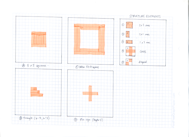
Now that we know 2 basic morphological operations, we go to the activity proper. The first part of the activity was to test our knowledge on erosion and dilation. We were tasked to illustrate by hand drawing the erosion and dilation of 4 different shapes using 5 different structure elements. The shapes are 
A. 5x5 square,
B. triangle with base = 4, height = 3 boxes,
C. hollow 10 x 10 square, 2 boxes thick, and 
D. plus sign, 1 box thick, and 5 boxes along each line.

The structuring elements are 
1. 2x2 ones,
2. 2x1 ones,
3. 1x2 ones, 
4. cross, 3 pixels long, 1 pixel thick, and 
5. a diagonal line (lower left to upper right), 2 boxes long.

These shapes and structuring elements are illustrated below

Shapes and structuring elements used

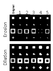
Now we perform erosion on the different shapes. Note that on the images, the letter denotes the shape being operated on and the number denotes the structuring element used. 

Erosion of the shapes

On the other hand, the following illustrations demonstrate dilation operation.

Dilation of the shapes

To verify whether our understanding of the erosion and dilation operations are correct, we use Scilab to perform these operations. These operations are available in the Image Processing Design toolbox of Scilab by calling ErodeImage and DilateImage functions. The resulting images are shown below. Again note that the numbers denote the structuring element used as labeled above. 

Erosion and dilation using Scilab

We observe that the results are the same when we use structuring elements 1 - 3, but differ when 4 and 5 are used. This is due to a difference in the set origin of the structuring element. The origin of the structuring element affects the resulting morphology after operation. In the case of the cross in Scilab, it seems that the origin was located at the center of the cross. For the diagonal, the origin was located a the lower left pixel of the diagonal. These can be deduced by observing the resulting images using structuring elements 4 and 5. 

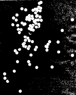
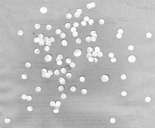
Now we are to apply morphological operations in processing images. We have below an image of simulated cells (punched holes) and what we want to do is obtain an estimate size of these cells. To start, we segment this image to determine the cells from the background.

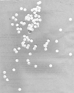Simulated cells

The histogram of the gray values in the image is shown below so that we can determine a threshold value to use. The values within the band correspond to the background of the image. We observe from the image that the cells are lighter than the background, so we deduce that the values greater than the band correspond to the cells. 

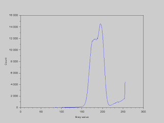Histogram of gray values

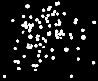
We set the threshold gray value to 210, and segment the image by using the function SegmentByThreshold. All values greater than this threshold are set to white and all values less than this threshold are set to black. The resulting image is shown below. 

Thresholded image

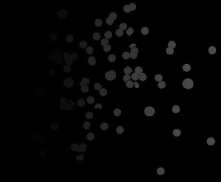
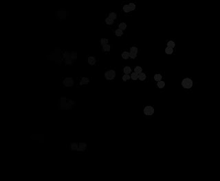
Here we see unwanted dots scattered in the image which are not cells. These are unwanted features in our segmented image. To remove these, we need to use morphological operations. We introduce another morphological operation -- opening. The opening operation is simply a combination of the operations we studied above. This operation involves eroding first the image and then dilating it. If we, for example, have a structuring element that is larger than a foreground region in the image, then erode the 2 images, the region completely turns into a background region. If we then perform dilation, the original foreground region would not be recovered. Effectively, with the opening operation, we can open gaps between the foreground pixels or we can see it as eliminating foreground pixels (http://homepages.inf.ed.ac.uk/rbf/HIPR2/open.htm). In our case, we use the OpenImage function using a circular structuring element with a radius of 4 pixels. The resulting image is shown below.

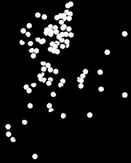Thresholded and cleaned image

We have now isolated the features we want to work with. The next thing we have to do is measure the sizes of each cell. To start, we identify each cell in our image, or blobs in general, and we do this by using the function SearchBlobs. What this does is label each blob with a number, and we can use that number to isolate that blob. At this point, when we use this function, we note that some of the cells are overlapping, which will effectively constitute a single blob. For the moment, we ignore this fact and calculate the area of each blob. The histogram of the blobs' areas (in pixels) are shown below.

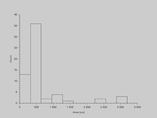Histogram of cell areas

To deal with this wide range of values for the areas, we use statistics! What we can do is determine the outliers in this data set and remove them. We can do this by using interquartile range (IQR). Outliers in a data set are those values (say \(x\)) which are \(x < Q_1 - 1.5IQR \) or \(x > Q_3 + 1.5IQR \), where \(Q_1\) is the 1st quartile, \(Q_3\) is the 3rd quartile, and \(IQR = Q_3 - Q_1\). After removing the outliers, the histogram results to the plot below. 

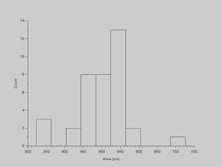Filtered histogram of cell areas

We can now calculate for an estimate of the cells' sizes. The mean is 501.08 and the standard deviation is 71.49. 

Now that we have an estimate of the cells' sizes, we can now go on to identify cancer cells among the normal cells. The image shown below contains normal cells and cancer cells. Initial steps in processing this image are the same for the previous image. We segment this image and clean it to remove the unwanted features. 

Simulated normal and cancer cells

Binarized image of the cells

We then identify the blobs in the image. The image below shows the identified blobs, where each blob denotes a different shade from the others. 

Image with identified blobs

Now, we use our estimate earlier to filter out the normal cells. We do this using the FilterBySize function. We set our threshold to a size of 501.08 + 71.49 = 572.57. When the size is lesser than this value, the blob is set to a background, and when the size is greater than this value, the blob is retained. We observe now that we are left with overlapping normal cells and abnormally large cells, which we deduce to be the cancer cells. 

Image with filtered blobs by size

Now, what we are left to do is to remove these overlapping normal cells, and to do this, we use the magic of the opening operation. We can create a structuring element that can remove these but not the cancer cells. In this case, a circular structuring element with a radius of 13 pixels is appropriate. The cancer cells are now successfully identified as shown below (binarized image).

Cancer cells

I would give myself a grade of 10 because I have done all of the stated tasks for this activity.