The FT is a linear transform which converts a signal in the spatial dimension to a signal in the reciprocal dimension (spatial frequency). The FT of a function \( f(x,y) \) is given by
$$F(f_x,f_y) = \iint f(x,y) \exp{[-i2\pi(f_xx + f_yy)]} dx dy$$
To implement this faster and more efficient, Cooley and Tukey developed an algorithm, the Fast Fourier transform (FFT), which is widely used in signal and image processing, and is usually readily available in different programming languages.
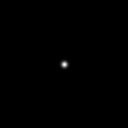
To get acquainted with the FFT, the first part of the activity involved implementation of FFT on different patterns. Firstly, we take FFT of a circle generated using Scilab. We do this by using the fft2() function in Scilab. Note that a characteristic of the FFT is that the pairs of quadrants of the image are interchaged. Quadrants 1 and 3 interchange, and quadrants 2 and 4 interchange as shown below.
 |
| Original orientation of quadrants |
 |
| Orientation of quadrants after FFT |
 |
| Circle generated using Scilab |
 |
| FFT of the circle |
 |
| FFT of the unshifted FFT of the circle |
Now, we consider an image of the letter A which was generated using Paint. We take the FFT of this image, and its FFT shifted spectrum is shown below. Now, if we take the FFT of the unshifted FFT of the image A, we get an inverted A. So it turns out, the circle earlier was inverted after all!
 |
| Letter A generated using Paint |
 |
| Shifted FFT spectrum of the letter A |
 |
| FFT of the unshifted FFT spectrum of the letter A |
Note that in the activity sheet, the 2nd FFT step was considered as an inverse FFT. This sparked a question in my mind. Is a 2nd FFT step equivalent to an inverse FFT? So I tried to inverse FFT the unshifted FFT of the letter A using the ifft() function of Scilab, and the result is shown below. We obtain back the original image! So we see now that the difference between a 2nd application of FFT and application of inverse FFT is the orientation of the resulting image. One is just a flipped (along the x-axis) image of the other.
 |
| Inverse FFT of the unshifted FFT spectrum of the letter A |
Different patterns to be FFT'd were also considered: corrogated roof, double slit, square function, and a 2D Gaussian curve. The patterns and their shifted FFT spectrum are shown below.
Corrogated roof pattern (left) and its FFT spectrum (right)
Double slit (left) and its FFT spectrum (right)
Square (left) and its FFT spectrum (right)
2D Gaussian curve (left) and its FFT spectrum (right)
Just some important points. The FFT of sinusoids produce peaks at the frequencies of these sinusoids. The brightest dots in the FFT of the corrogated roof correspond to the \( \pm \) frequencies of the sinusoid. The intensities near these values are due to the flat portion of the pattern (the black portions), or in general, abrupt changes of values (edges). Note that the generated sinusoid contains negative values. But when these are to be rendered as images, the negative values assigned as zeros. Now for the square pattern, we can imagine it as a sinusoid with 0 frequency, so the main peak is at the 0 point, and the following decreasing intensities along the x and y axes are due to the same reasons as earlier (i.e. the presence of edges). Finally, we note the equation for the Fourier transform of a function, and see that if our function is an exponential, then the results will still be an exponential. And so, the FT of a Gaussian function is also Gaussian. Here are some links to serve as reference:
The next part of the actiivity involves convolution. If we have 2 functions \( f(x,y) \) and \( g(x,y) \), and we take their convolution to obtain \( h(x,y) \), we have the relation
$$\iint f(x',y') g(x-x',y-y') dx' dy'$$
If \( H,F,G \) are the FT of \( h,f,g\) respectively, then following the convolution theorem, we have the relation
$$ H = FG $$
Convolution sort of mixes 2 functions with each other. Using the words of the discussion in the activity sheet, it smears functions against each other. And using the words from the Wolfram site(http://mathworld.wolfram.com/Convolution.html), it blends one function with another. With this characteristic of convolution, it may be used to simulate a simple lens setup, which we do in this activity. To serve as our object, an image of the acronym VIP (shown below) was created using Paint. Circles of different radii were also generated in Scilab to serve as our apertures in our simulations. These were convolved by taking the FFT of the VIP image, FFT shifting the image of the aperture (since it is in the fourier plane), and multiplying them element-wise. This follows from the convolution theorem. Finally, we perform inverse FFT to obtain the resulting image. The apertures and the resulting images are shown below, where the resulting images are beside their corresponding apertures.
 |
| Image of VIP created using Paint |
The resulting images of VIP beside their corresponding aperture
We can see that using the smallest aperture, we have a blurred image. As we increase the aperture size, the image becomes clearer and more resolved. We expect this trend since if we have a larger aperture, we have more passing light rays (more information), and so we obtain a better resolved image of the object.
Now, we turn to another concept -- correlation. If \( p(x,y) \) is the correlation between the functions \( f,g \), then these functions are related by
$$p(x,y) = \iint f(x',y') g(x+x',y+y') dx' dy'$$
Similar to the convolution theorem, the correlation theorem states that if \( P,F,G \) are the FT's of \( p,f,g \), these are related by
$$P = F^*G$$
where \(^*\) denotes complex conjugation.
Correlation helps in template matching since it measures, well, as the name suggests, the degree of correlation or similarity between 2 functions. Correlation is high if we have a high degree of similarity and correlation is low if the 2 functions are not quite similar.
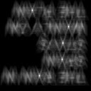
For this part of the activity, we have as our object an image of the statement "THE RAIN IN SPAIN STAYS MAINLY ON THE PLAIN". Then, we also create an image of the letter A with the same font and font size as the statement. And now, here comes the magical part of correlation. If we take the conjugate of the FFT of letter A, multiply it to the FFT of the statement, and inverse FFT the product, we get a similar image of the statement, but not as resolved as the original image.
 |
| Image of a statement to serve as our object |
Image of a letter A (left) and the resulting correlation with the statement image (right)
This got me thinking, what if the letter A was not the same size as that in the statement? What if A was bigger, and what if A was smaller? The resulting correlations are shown below.
Image of the letter A's (left) and their corresponding correlations with the statement (right)
We see that with a larger A, the resulting correlation is blurred. We can't even read the statement. However, if we have a smaller A, we see a more resolved correlation. This is even more resolved than that when the A was of the same size as that in the statement.
Another question that entered my mind: does the position of letter A matter? What if we move it off center? So I placed the letter A at the upper left corner and the resulting correlation is shown below.
Image of the letter A at the upper left (left) and its corresponding correlation with the statement (right)
It turns out, it does have an effect! The position of the resulting correlation depends on the position of the letter A. Since the letter A was moved towards the upper left, the correlation was also moved towards the upper left.
Finally, we apply template matching for the purpose of edge detection (which reminds me of the activity 4 since we used the edge function of Scilab!). We again consider the image of the VIP acronym. We then create 9x9 images of different patterns: vertical edge, horizontal edge, spot, and X pattern. Note that the sum of the matrix values must sum to 0. The VIP image and the patterns were then convolved using conv2(). The resulting images are shown below.
Images after convolution using the following templates (from left to right): horizontal edge, vertical edge, spot, and X pattern.
We note that we indeed match the 2 images. Observe that when we use the horizontal edge template, the vertical edge of I and P are not visible! A similar observation can be seen when using the vertical edge. We see that the template is considered as the smallest element of an edge to be matched with the image (reminds me of a crystal! the template is like a unit cell, which repeats periodically in a crystal). We also observe this characteristic when we use the spot and X patterns.
Finally, we are done! That was quite interesting despite the many lines of coding and quantity of images. With this activity, we have been introduced to the power of the FT (or the FFT) in image processing. Again, I have come to know more on the applications of the concepts that we have been learning in our Physics courses. I would give myself a grade of 10, since I was able to perform all of the tasks in the activity and report the results here in this blog.
I have included the code which I used in this activity for the benefit of those who want to replicate the same or similar results.
FFT of different patterns
1 2 3 4 5 6 7 8 9 10 11 12 13 14 15 16 17 18 19 20 21 22 23 24 25 26 27 28 29 30 31 32 33 34 35 36 37 38 39 40 | x = linspace(-1,1,128); y = linspace(-1,1,128); [X,Y] = ndgrid(x,y); // Circle circle = zeros(128,128); r = sqrt(X.^2 + Y.^2); circle(find(r<0.4)) = 1; // Letter A A = imread('C:\Users\toshiba\Google Drive\College\5th year\App Physics 186\Act5\A.bmp') // Sinusoid along the x sine = sin(30*Y); // Double slit dslit = zeros(128,128); dslit(51:78,50) = 1; dslit(51:78, 79) = 1; // Square sq = zeros(128,128); sq(35:94,35:94) = 1; // 2D Gaussian Bell curve r2 = X.^2 + Y.^2; gauss = exp(-r2/0.05); function FFTshape=FFT(shape) Fshape = fft2(double(shape)); FFTshape = uint8(255*(abs(fftshift(Fshape))/max(abs(fftshift(Fshape))))); imshow(FFTshape); endfunction function FFTFFTshape=FFTFFT(shape) FFshape = fft2(fft2(double(shape))); FFTFFTshape = uint8(255*((abs(FFshape))/max(abs(FFshape)))); imshow(FFTFFTshape); endfunction |
Convolution (simple lens setup)
1 2 3 4 5 6 7 8 9 10 11 12 | circle = imread('C:\Users\toshiba\Google Drive\College\5th year\App Physics 186\Act5\circle09.bmp'); VIP = imread('C:\Users\toshiba\Google Drive\College\5th year\App Physics 186\Act5\VIP.bmp'); Fcircle = fftshift(double(circle)); FVIP = fft2(double(VIP)); circle_VIP_convol = Fcircle .* FVIP; inv_circle_VIP_convol = ifft(circle_VIP_convol); VIP_convol_im = uint8(255*(abs(inv_circle_VIP_convol)/max(abs(inv_circle_VIP_convol)))) //imshow(VIP_convol_im); //imwrite(VIP_convol_im, 'C:\Users\toshiba\Google Drive\College\5th year\App Physics 186\Act5\VIP_convol_im_09.bmp') |
Correlation (template matching)
1 2 3 4 5 6 7 8 9 10 11 12 | statement = imread('C:\Users\toshiba\Google Drive\College\5th year\App Physics 186\Act5\statement2.bmp'); A = imread('C:\Users\toshiba\Google Drive\College\5th year\App Physics 186\Act5\A2-2small.bmp'); Fstatement = fft2(double(statement)); FA = fft2(double(A)); correlation = FA .* conj(Fstatement); inv_correlation = fftshift(ifft(correlation)); inv_correlation_im = uint8(255*(abs(inv_correlation)/max(abs(inv_correlation)))); //imshow(inv_correlation_im); //imwrite(inv_correlation_im, 'C:\Users\toshiba\Google Drive\College\5th year\App Physics 186\Act5\A2-2small-corr.bmp'); |
Edge detection
1 2 3 4 5 6 7 8 9 10 11 12 13 14 15 16 17 18 | hedge = [-1,-1,-1 ; 2,2,2 ; -1,-1,-1]; //horizontal edge vedge = [-1,2,-1 ; -1,2,-1 ; -1,2,-1]; // vertical edge spot = [-1,-1,-1 ; -1,8,-1 ; -1,-1,-1]; // spot X = [-4,5,-4 ; 5,-4,5 ; -4,5,-4]; // X pattern VIP = imread('C:\Users\toshiba\Google Drive\College\5th year\App Physics 186\Act5\VIP.bmp'); VIP_hedge = conv2(double(VIP),double(hedge)); imwrite(VIP_hedge,'C:\Users\toshiba\Google Drive\College\5th year\App Physics 186\Act5\VIP_hedge.bmp'); VIP_vedge = conv2(double(VIP),double(vedge)); imwrite(VIP_vedge,'C:\Users\toshiba\Google Drive\College\5th year\App Physics 186\Act5\VIP_vedge.bmp'); VIP_spot = conv2(double(VIP),double(spot)); imwrite(VIP_spot,'C:\Users\toshiba\Google Drive\College\5th year\App Physics 186\Act5\VIP_spot.bmp'); VIP_X = conv2(double(VIP),double(X)); imwrite(VIP_X,'C:\Users\toshiba\Google Drive\College\5th year\App Physics 186\Act5\VIP_X.bmp'); |


No comments:
Post a Comment