Activity 6 is again all about the Fourier transform (FT). So BEWARE: FFT OVERLOAD all over again! This time, we further explore the properties of FFT, and take note of these as we use FFT in different applications.
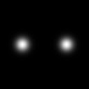
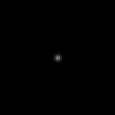
For the first part of the activity, we explore the anamorphic property of FT. Note that when performing FT, we transfer from a spatial dimension (say \( x \) ) to a spatial frequency dimension (\( k_x \)), which is basically an inverse dimension of \( x \). Here, we have different 2D patterns: tall rectangle, wide rectangle, and 2 centrally symmetric dots (along the x-axis) with different separation distances. The patterns are shown below along with their FFT's.
Synthesized patterns (left) and their FFT spectra (right)
Note that for the tall rectangle, we get an FFT that is wide (or stretched along the horizontal). On the other hand, if we consider the wide rectangle, we get wallt features in the FFT spectrum (stretched along the vertical). This exhibits the anamorphism brought about by the FT, where a long dimension in space is a shorter dimension in the Fourier space, and a short dimension in space is a longer dimension in the Fourier space.
Now, we focus on sinusoid signals and their FFT's. First we start with sinusoids with different frequencies. 2D images of sinusoids along the horizontal were generated, varying the frequencies of each. FFT was then performed on each of these sinusoid signals. The images and FFT spectra are shown below.
Sinusoids with increasing frequency from top to bottom (left) and their corresponding FFT spectra (right)
In the past activity, we have already discussed the FFT of the same pattern, and so this is sort of just a review. We have already learned that the FFT of a sinusoid is a peak at the corresponding \( \pm \) frequencies of the sinusoid. And so, since our sinusoid is along the horizontal, we expect that our peaks are located along the horizontal. Also, as the frequency of the sinusoid is increased, it is expected that the peaks move farther away from the center, which we indeed see in the generated FFT spectra above.
Now, suppose that we add a constant bias to the sinusoid and we take its FFT. The image and its FFT spectrum is shown below.
Sinusoid with constant bias (left) and its FFT spectrum (right)
Since we only added a constant to the sinusoid signal, we expect to see the characteristic peaks associated with the sinusoid signal. The difference which we see is the peak at the center of the spectrum? If we consider the same concept as that with sinusoids, where the FFT shows the frequency of the sinusoid, then in this case we have a signal with 0 frequency, which we can deduce to be the constant added.
Now, instead of limiting ourselves to a sinusoid along the horizontal, we rotate the sinusoid along the center to have some variation (and of course to see what happens to the FFT spectrum). The sinusoids were rotated by considering the following form of a sinusoid to be \( \sin{(2\pi f (Y\sin{\theta} + X\cos{\theta}))} \), where \( \theta \) controls the degree of rotation of the sinusoid. The images of the sinusoids and its corresponding FFT spectra are shown below.
Rotated sinusoids with increasing \(\theta\) (left) and their corresponding FFT spectra (right)
Note that the FFT spectrum also seems to rotate! Although, we should not be that shocked since this is just similar to that when the sinusoid was along the horizontal. The peaks of the FFT lie on the same line as where the sinusoids are propagating. If we look at the equation of the rotated sinusoid, we note that the frequency is as if being broken down into components( \( f\sin{\theta} and f\cos{\theta} \) ).
Next, we consider multiplied sinusoids along the x and along the y. This is of the form \( \sin{(2\pi f_xX)} \sin{(2\pi f_yY)} \). The resulting images are shown below , along with their corresponding FFT spectra. From top to bottom, the frequencies of the sinusoid along the horizontal are increasing.
Multiplied sinusoids with increasing ferquency along the horizontal from top to bottom (left) and their corresponding FFT spectra (right)
Coool, we get checkerboard-like patterns. Note that in the FFT spectra, we already have 4 peaks. These 4 peaks arise because of the multiplication of the sinusoids. To understand this, we review our trigonometry. If we have the product of sines considered above, we can decompose it into a sum using the formula (taken from http://www.sosmath.com/trig/prodform/prodform.html)
$$\sin{a} \sin{b} = \dfrac{1}{2} \left( \cos{(a-b)} - \cos{(a+b)} \right)$$
And so, we have
$$ \sin{(2\pi f_x X)} \sin{(2\pi f_y Y)} = \dfrac{1}{2} \left\{ \cos{[2\pi (f_xX - f_yY)]} - \cos{[2\pi (f_xX + f_yY)]} \right\} $$
Note that the right side of the equation has 2 sinusoids, each with the same form as a rotated sinusoid, which explains why we get the 4 peaks in the FFT spectrum since addition of sinusoids only superposes the individual FFT's into a single spectrum.
The following patterns are sort of just for fun. We add different combinations of sinusoids (multiplied and rotated) to form different cool and visually appealing patterns. Again, since we are adding the sinusoids, then we expect that the FFT spectrum will be a superposition of the individual FFT's of the addends. The resulting images of combinations of sinusoids and their FFT's are shown below (I don't know why but when I see these I see snakes, worms.... and french fries :) ).
Combinations of sinusoids (left) and their FFT spectra (right)
For the next part, we were tasked to create 2 dirac deltas symmetric about the center. and take its FFT. The image and the FFT spectrum is shown below. Based on the analytical FT of a dirac delta function, the result is a complex exponential(http://mathworld.wolfram.com/FourierTransformDeltaFunction.html), so we expect this periodic FFT spectrum. 2 circles symmetric about the center were also produced, varying the radii of the circle, and the FFT spectra were computed. Note that if we increase the radii of the circles, the size of the central peak of the corresponding FFT decreases, which is brought about by the anamorphic property of the FFT. A common characteristic among all the the FFT's is the presence of a fringe-like pattern. The resulting FFT spectrum can actually be explained using the convolution theorem. The convolution theorem states that a convolution in space is equivalent to a product in the Fourier space. Also, a convolution of a dirac delta function with another function results to the function being shifted to the position of the dirac delta. In our case, the image of the 2 circles can be thought of as a convolution of 2 dirac delta functions and a circle. If we then take its FFT, by the convolutiong theorem, we expect that the resulting FFT is a product of the individual FFT's. The FFT of the dirac delta functions is shown below, and the FFT of a circle is a Bessel function of the 1st kind (as discussed in Activity 5), and so the product of these are shown below for different radii of the circle.


2 dirac delta functions (left) and its FFT spectrum (right)
2 circular patterns (left) and the corresponding FFT spectra (right)
Then I asked, what if the 2 circles did not have the same radii? So I tried to generate an image and take its FFT, and the images are shown below. There is not much of a difference except that the fringes are not vertical anymore. It seem that the fringes are already curved. To understand this, we note the image may be thought of as a superposition of 2 convolutions: (a) dirac delta and a circle, (b) dirac delta and a circle with greater radius. And so, if we take the FT of this, the spectrum will be the superposition of the individual FT's of (a) and (b). Essentially, the difference in the radii brings about a difference in the size of the airy pattern produced, producing the FFT spectrum below.
2 circles with different radii (left) and its corresponding FFT spectrum (right)
The same was done, although this time using a Gaussian profile. The images and the FFT spectra are shown below, with increasing variance from top to bottom. Note that previously, we have learned that the FFT of a Gaussian is still a Gaussian, so we get the FFT spectra below, superposed with the FFT spectrum of 2 dirac delta functions. Again, we see the anamorphic property of the FT since we observe that as the width of the Gaussian is increased, the width of the resulting Gaussian decreases.
2 Gaussian profiles (left) and their corresponding FFT spectra (right)
Out of curiosity at the time of the activity, I also did the same procedure, but with squares. I didn't know that time that the results would simply be just the superposition of the individual FT's. But now, it looks so basic (which is good! A sign of new knowledge).
2 squares (left) and their corresponding FFT spectra (right)
The next part of the activity involved placing dirac delta functions in random positions, and convolving different 3x3 patterns with these. In this case, the patterns I tried were: box, horizontal line, vertical line, letter 'I', and letter 'X'. As we have mentioned earlier, a convolution with a dirac delta function results to a replication (or an imagined photocopy) of the convolved function on to the position of the dirac delta, which we see in the images below.
10 randomly placed dirac delta functions convolved with different patterns.
For the next part, instead of placing dirac delta functions randomly, these were positioned with uniform distances between each other, and the separation distance was increased, as shown below. FFT was performed on each one, and their corresponding FFT spectra are shown below, beside the images. Again, we note that the FFT of a dirac delta function is a complex exponential. If we have dirac delta functions along the horizontal, we expect the FFT to progress along the horizontal. The same goes for the vertical direction. The distance of the dirac delta from the center denotes the frequency in the exponent of the complex exponential. And so, the FFT is basically a superposition of complex exponentials with harmonic frequencies, giving rise to the FFT spectra below. Again, we see here the anamorphic property of FT. The closer the dirac delta functions are spaced, the larger the pattern formed. Or alternatively, we may also think of the image as zoomed out, and the FFT as zoomed in. As we zoom in to the groupd of dirac delta functions, we zoom out of the FFT spectrum.


Equally spaced dirac delta functions with increasing spacing from top to bottom (left) and their corresponding FFT spectra (right)
Next, we use FFT on a fingerprint. In fingerprints, sometimes there are discontinuous ridges and blotches which we do not want. We want the ridges to be continuous and not be blocked by these blotches. To do this, we use the power of FFT. An image of my thumbmark is shown below.
 |
| Image of a thumbmark |
We then take the FFT of this image, which is shown below. We notice an elliptical-like feature in the FFT spectrum, and 4 peaks corresponding to rotated sunusoids. We suspect these features to correspond to the ridges of the thumbmark. And so, we create a mask which we are to convolve with the FFT spectrum, to retain these features and wipeout all others. The mask is shown below.
FFT spectrum of the thumbmark in log scale (left) and the created mask (right)
If we convolve these 2 images, we get the image of the thumbmark below. Although the image seems blurred (due to the filtered out part in the FFT), we can see that the blotches are suppressed. With the suppression of these blotches, the ridges become continuous. Also notice that in the original image (top right portion) the ridges are discontinuous, while in the processed image, we see the ridges to be extended.
 |
| Processed image of the thumbmark |
Now, we apply the FFT so as to remove unwanted features in an image. Shown below is an image of a part of the moon. We can see regularly spaced horizontal lines in the image, which we do not want in the image. We exploit FFT in this case for us to remove these features. The FFT spectrum is shown below.
 |
| Image of a part of the moon with horizontal line features |
 |
| FFT spectrum (in log scale) of the image of the moon |
Let's work with what we know. If the features are horizontal lines, then by the anamorphic property of FT, we expect the FFT spectrum to have high values along the vertical. We indeed see this in the FFT spectrum above, and so we need to suppress these. We block off these white signals along the vertical (along the center) except for the central peak which corresponds to the DC peak (to prevent the image from getting darker), as shown below
 |
| Edited FFT spectrum of the image of the moon |
We then perform inverse FFT, and voila! The horizontal lines disappear! The cleaned image is shown below.
We also exploit FFT in processing images of a painting on canvas. A sample image is shown below
 |
| Colored painting |
 |
| Black and white version of the painting |
Our goal here is to remove the features of the canvas. Note that the canvas is more or less uniform across the image, and is a regular and repetitive pattern. And so, the weave pattern may be thought of as a superposition of different combinations of sinusoids. The FFT spectrum of the image indeed shows this since we see a lot of peaks.
 |
| FFT spectrum (in log scale) of the painting |
What we need to do is suppress these peaks to somehow delete the information of the canvas. We can do this by creating a mask with white background and black squares on the locations of the peaks. The locations of the peaks were determined using Paint, and the mask was produced using Scilab. The mask can then be convolved with the FFT spectrum of the image, and the resulting spectrum be inverse FFT'd to obtain the cleaned image. To also determine the filtered out part of the image, the mask was inverted (white became black and black became white), convolved with the FFT of the image, and inverse FFT'd. The filter, filtered image, and filtered out part of the image are shown below for increasing size of the black squares in the filter.
(a)
(b)
(c)
Images of the filter, filtered image, and filtered out part of the image, with increasing size of black squares from (a) to (c)
Note that for (a), we have already removed most of the canvas features. As the black squares are increased, further removal of the canvas can be observed. However, the images of the filtered out portions progress to form an image of the house. This is greatly exhibited in (c). We almost see defined boundaries of the house being filtered out of the original image, which we do not want. What we want is a maximum removal of the canvas and minimal removal of the main painting's features. So, it is not a good idea to have very large filters of the FFT peaks. (b) shows a quite good balance between the removal of the canvas and painting's features. Most canvas features have already been removed while maintaining minimal removal of the painting's features.
If you reached this point without skipping any of the discussions above, I applaud you! Standing ovation! Slow clap! Because that was a very long blog all about FFT. Despite the overwhelming quantity of tasks in this activity, it was very interesting. I enjoyed more especially those which involved editing images using the FFT, because before, I never thought of the FFT to be that powerful. Because of this, I learned to do magic! Or i mean, 'magic' :). Before I forget, I would like to thank Carlo and Mich for the healthy discussions regarding this activity. Our discussions helped in achieving the desired results of this activity. The activity sheet prepared by ma'am also is a big help in preparing this blog. I would give myself a grade of 10. I did my best in all of the parts of the activity, reported them in this blog, and have learned a lot while doing this activity.
The code for the different parts of the activity are shown below for the reader's reference.
Exploration of the anamorphic property of FT
1
2
3
4
5
6
7
8
9
10
11
12
13
14
15
16
17
18
19
20
21
22
23
24
25
26
27
28
29
30
31
32
33
34
35
36
37
38
39
40
41
42
43
44
45
46
47
| nx = 128; ny = 128
x = linspace(-1,1,nx);
y = linspace(-1,1,ny);
[X,Y] = ndgrid(x,y);
// Tall rectangle
t_rect = zeros(nx,ny);
t_rect((1/4)*nx:(3/4)*nx,(3/8)*ny:(5/8)*ny) = 1;
//imshow(t_rect);
//imwrite(t_rect,'C:\Users\csrc-lab03\Documents\gelo\Act6\t_rect.bmp');
Ft_rect = fft2(t_rect);
Ft_rect_im = uint8(255*abs(fftshift(Ft_rect))/max(abs(fftshift(Ft_rect))));
imshow(Ft_rect_im);
imwrite(Ft_rect_im,'C:\Users\csrc-lab03\Documents\gelo\Act6\Ft_rect.bmp');
// Wide rectangle
w_rect = zeros(nx,ny);
w_rect((3/8)*nx:(5/8)*nx,(1/4)*ny:(3/4)*ny) = 1;
//imshow(w_rect);
//imwrite(w_rect,'C:\Users\csrc-lab03\Documents\gelo\Act6\w_rect.bmp');
Fw_rect = fft2(w_rect);
Fw_rect_im = uint8(255*abs(fftshift(Fw_rect))/max(abs(fftshift(Fw_rect))));
imshow(Fw_rect_im);
imwrite(Fw_rect_im,'C:\Users\csrc-lab03\Documents\gelo\Act6\Fw_rect.bmp');
// 2 dots along x-axis
dots = zeros(nx,ny);
dots(nx/2,3*ny/8) = 1;
dots(nx/2,5*ny/8) = 1;
//imshow(dots);
//imwrite(dots,'C:\Users\csrc-lab03\Documents\gelo\Act6\dots.bmp');
Fdots = fft2(dots);
Fdots_im = uint8(255*abs(fftshift(Fdots))/max(abs(fftshift(Fdots))));
imshow(Fdots_im);
imwrite(Fdots_im,'C:\Users\csrc-lab03\Documents\gelo\Act6\Fdots.bmp');
// 2 dots along x-axis with wider distance
dots2 = zeros(nx,ny);
dots2(nx/2,1*ny/8) = 1;
dots2(nx/2,7*ny/8) = 1;
//imshow(dots2);
//imwrite(dots2,'C:\Users\csrc-lab03\Documents\gelo\Act6\dots2.bmp');
Fdots2 = fft2(dots2);
Fdots2_im = uint8(255*abs(fftshift(Fdots2))/max(abs(fftshift(Fdots2))));
imshow(Fdots2_im);
imwrite(Fdots_im,'C:\Users\csrc-lab03\Documents\gelo\Act6\Fdots2.bmp');
|
FFT of sinusoids
1
2
3
4
5
6
7
8
9
10
11
12
13
14
15
16
17
18
19
20
21
22
23
24
25
26
27
28
29
30
31
32
33
34
35
36
37
38
39
40
41
42
43
44
45
46
47
48
49
50
51
52
53
54
55
56
57
58
| x = linspace(-1,1,128);
y = linspace(-1,1,128);
[X,Y] = ndgrid(x,y);
// Sinusoid along the x
f = 5;
sine = sin(2*%pi*f*Y) + 2;
imshow(sine);
imwrite(sine,'C:\Users\csrc-lab03\Documents\gelo\Act6\sine_f'+string(f)+'.bmp');
Fsine = fft2(double(sine));
Fsine_im = uint8(255*abs(fftshift(Fsine))/max(abs(fftshift(Fsine))));
imshow(Fsine_im);
imwrite(Fsine_im,'C:\Users\csrc-lab03\Documents\gelo\Act6\Fsine_f'+string(f)+'.bmp');
// Rotated sinusoid
f2 = 5;
theta = 5*%pi/6;
rotsine = sin(2*%pi*f2*(Y*sin(theta) + X*cos(theta)));
imshow(rotsine);
imwrite(rotsine,'C:\Users\csrc-lab03\Documents\gelo\Act6\rotsine_theta'+string(theta)+'.bmp')
Frotsine = fft2(rotsine);
Frotsine_im = uint8(255*abs(fftshift(Frotsine))/max(abs(fftshift(Frotsine))));
imshow(Frotsine_im);
imwrite(Frotsine_im,'C:\Users\csrc-lab03\Documents\gelo\Act6\Frotsine_theta'+string(theta)+'.bmp');
// Element-wise multiplied sinusoids
F1 = 5; F2 = 20;
sine1 = sin(2*%pi*F1*X);
sine2 = sin(2*%pi*F2*Y);
msine = sine1 .* sine2;
imshow(msine);
imwrite(msine,'C:\Users\csrc-lab03\Documents\gelo\Act6\msine_F1_' + string(F1) + '_F2_' + string(F2) + '.bmp');
Fmsine = fft2(msine);
Fmsine_im = uint8(255*abs(fftshift(Fmsine))/max(abs(fftshift(Fmsine))));
imshow(Fmsine_im);
imwrite(Fmsine_im,'C:\Users\csrc-lab03\Documents\gelo\Act6\Fmsine_F1__' + string(F1) + '_F2_' + string(F2) + '.bmp');
// Element-wise multiplied sinusoids + rotated sinusoids
F1 = 5; F2 = 20;
SINE1 = sin(2*%pi*F1*X);
SINE2 = sin(2*%pi*F2*Y);
F3 = 5;
theta2 = %pi/2;
SINE3 = sin(2*%pi*F3*(Y*sin(theta2) + X*cos(theta2)));
SINE = SINE1 .* SINE2 + SINE3;
imshow(SINE);
imwrite(SINE,'C:\Users\csrc-lab03\Documents\gelo\Act6\SINE_F1_' + string(F1) + '_F2_' + string(F2) + '_F3_' + string(F3) + '_theta_' + string(theta2) + '.bmp');
FSINE = fft2(SINE);
FSINE_im = uint8(255*abs(fftshift(FSINE))/max(abs(fftshift(FSINE))));
imshow(FSINE_im);
imwrite(FSINE_im,'C:\Users\csrc-lab03\Documents\gelo\Act6\FSINE_F1_' + string(F1) + '_F2_' + string(F2) + '_F3_' + string(F3) + '_theta_' + string(theta2) + '.bmp')
|
Convolution and dirac delta functions
 1
 2
 3
 4
 5
 6
 7
 8
 9
10
11
12
13
14
15
16
17
18
19
20
21
22
23
24
25
26
27
28
29
30
31
32
33
34
35
36
37
38
39
40
41
42
43
44
45
46
47
48
49
50
51
52
53
54
55
56
57
58
59
60
61
62
63
64
65
66
67
68
69
70
71
72
73
74
75
76
77
78
79
80
81
82
83
84
85
86
87
88
89
90
91
92
93
94
95
96
97
98
99
100
101
102
103
104
105
106
107
108
109
110
111
| nx = 128; ny = 128;
x = linspace(-1,1,nx);
y = linspace(-1,1,ny);
[X,Y] = ndgrid(x,y);
// 2 dots
dots = zeros(nx,ny);
dots(nx/2,ny/4) = 1;
dots(nx/2,3*ny/4) = 1;
imshow(dots);
imwrite(dots,'C:\Users\csrc-lab03\Documents\gelo\Act6\Act6Cdots.bmp');
Fdots = fft2(dots);
Fdots_im = uint8(255*abs(fftshift(Fdots))/max(abs(fftshift(Fdots))));
imshow(Fdots_im);
imwrite(Fdots_im,'C:\Users\csrc-lab03\Documents\gelo\Act6\Act6CFdots.bmp');
// 2 circles
circles = zeros(nx,ny);
r1 = sqrt(X.^2 + (Y-.5).^2);
r2 = sqrt(X.^2 + (Y+.5).^2);
r1max = 0.4; r2max = 0.4;
circles(find(r1<r1max)) = 1;
circles(find(r2<r2max)) = 1;
imshow(circles);
imwrite(circles,'C:\Users\csrc-lab03\Documents\gelo\Act6\circles_r1_' + string(r1max) + '_r2_' + string(r2max) + '.bmp');
Fcircles = fft2(circles);
Fcircles_im = uint8(255*abs(fftshift(Fcircles))/max(abs(fftshift(Fcircles))));
imshow(Fcircles_im);
imwrite(Fcircles_im,'C:\Users\csrc-lab03\Documents\gelo\Act6\Fcircles_r1_' + string(r1max) + '_r2_' + string(r2max) + '.bmp');
// 2 squares
squares = zeros(nx,ny);
wx = 10; wy = 10;
squares(nx/2 - wx/2:nx/2 + wx/2 , ny/4 - wy/2 : ny/4 + wy/2) = 1;
squares(nx/2 - wx/2:nx/2 + wx/2 , 3*ny/4 - wy/2 : 3*ny/4 + wy/2) = 1;
imshow(squares);
imwrite(squares,'C:\Users\csrc-lab03\Documents\gelo\Act6\squares_wx_' + string(wx) + '_wy_' + string(wy) + '.bmp');
Fsquares = fft2(squares);
Fsquares_im = uint8(255*abs(fftshift(Fsquares))/max(abs(fftshift(Fsquares))));
imshow(Fsquares_im);
imwrite(Fsquares_im,'C:\Users\csrc-lab03\Documents\gelo\Act6\Fsquares_wx_' + string(wx) + '_wy_' + string(wy) + '.bmp');
// 2 gaussians
sigma2 = 0.06;
R1 = X.^2 + (Y-.5).^2;
gauss1 = exp(-R1/sigma2);
sigma22 = 0.01;
R2 = X.^2 + (Y+.5).^2;
gauss2 = exp(-R2/sigma22);
gauss = gauss1 + gauss2;
imshow(gauss);
imwrite(gauss,'C:\Users\toshiba\Google Drive\College\5th year\App Physics 186\Act6\gauss_sigma2_' + string(sigma2) + '_sigma22_' + string(sigma22) + '.bmp');
Fgauss = fft2(gauss);
Fgauss_im = uint8(255*abs(fftshift(Fgauss))/max(abs(fftshift(Fgauss))));
imshow(Fgauss_im);
imwrite(Fgauss_im,'C:\Users\toshiba\Google Drive\College\5th year\App Physics 186\Act6\Fgauss_sigma2_' + string(sigma2) + '_sigma22_' + string(sigma22) + '.bmp');
Randomly placed 1's
A = zeros(200,200);
for i = 1:10
A(uint8(rand()*200),uint8(rand()*200)) = 1;
end
xmark = [1,0,1;0,1,0;1,0,1];
Axmark = conv2(A,xmark);
imshow(Axmark);
imwrite(Axmark,'C:\Users\toshiba\Google Drive\College\5th year\App Physics 186\Act6\Axmark.bmp');
vert = [0,1,0;0,1,0;0,1,0];
Avert = conv2(A,vert);
imshow(Avert);
imwrite(Avert,'C:\Users\toshiba\Google Drive\College\5th year\App Physics 186\Act6\Avert.bmp');
hor = [0,0,0;1,1,1;0,0,0];
Ahor = conv2(A,hor);
imshow(Ahor);
imwrite(Ahor,'C:\Users\toshiba\Google Drive\College\5th year\App Physics 186\Act6\Ahor.bmp');
I = [1,1,1;0,1,0;1,1,1];
AI = conv2(A,I);
imshow(AI);
imwrite(AI,'C:\Users\toshiba\Google Drive\College\5th year\App Physics 186\Act6\AI.bmp');
box = [1,1,1;1,0,1;1,1,1];
Abox = conv2(A,box)
imshow(Abox);
imwrite(Abox,'C:\Users\toshiba\Google Drive\College\5th year\App Physics 186\Act6\Abox.bmp');
// Equally spaced 1's
B = zeros(200,200);
space = 3;
B(100,[100-3*space, 100-2*space, 100-space,100,100+space,100+2*space,100+3*space]) = 1;
B([100-3*space, 100-2*space, 100-space,100,100+space,100+2*space,100+3*space],100) = 1;
imshow(B);
imwrite(B,'C:\Users\toshiba\Google Drive\College\5th year\App Physics 186\Act6\B_space_' + string(space) + '.bmp');
FB = fft2(B);
FB_im = uint8(255*abs(fftshift(FB))/max(abs(fftshift(FB))));
imshow(FB_im);
imwrite(FB_im,'C:\Users\toshiba\Google Drive\College\5th year\App Physics 186\Act6\FB_space_' + string(space) + '.bmp');
|
Ridge enhancement of fingerprint
1
2
3
4
5
6
7
8
9
10
11
12
13
14
15
16
17
18
19
| thumb = imread('C:\Users\toshiba\Google Drive\College\5th year\App Physics 186\Act6\thumbmark.jpeg');
thumb = rgb2gray(thumb);
//imshow(thumb);
Fthumb = fft2(double(thumb));
Fthumb_shift = fftshift(Fthumb);
Fthumb_im = uint8(255*abs(Fthumb_shift)/max(abs(Fthumb_shift)));
Fthumb_im_log = uint8(255*log(abs(Fthumb_shift))/max(log(abs(Fthumb_shift))));
//imshow(Fthumb_im_log);
//imwrite(Fthumb_im_log,'C:\Users\toshiba\Google Drive\College\5th year\App Physics 186\Act6\Fthumbmark.jpg')
mask = imread('C:\Users\toshiba\Google Drive\College\5th year\App Physics 186\Act6\Fthumbmark_mask5.jpg');
mask = double(rgb2gray(mask));
Fthumb_mask = Fthumb_shift .* mask;
Fthumb_mask_invshift = ifft(fftshift(Fthumb_mask));
thumb_edited = uint8(255*abs(Fthumb_mask_invshift)/max(abs(Fthumb_mask_invshift)));
//imshow(thumb_edited);
//imwrite(thumb_edited,'C:\Users\toshiba\Google Drive\College\5th year\App Physics 186\Act6\thumb-edited.jpg');
|
Removal of horizontal lines in lunar image
1
2
3
4
5
6
7
8
9
10
11
12
13
14
15
16
17
18
19
20
21
22
23
24
25
| lunar = imread('C:\Users\csrc-lab03\Documents\gelo\Act6\Act6-lunar.jpg');
//imshow(lunar);
Flunar = fft2(double(lunar));
Flunar_shift = fftshift(Flunar);
Flunar_im = uint8(255*abs(Flunar_shift)/max(abs(Flunar_shift)));
Flunar_im_log = uint8(255*log(abs(Flunar_shift))/max(log(abs(Flunar_shift))));
//imshow(Flunar_im_log);
//imwrite(Flunar_im_log,'C:\Users\csrc-lab03\Documents\gelo\Act6\Act6-lunar-FFTlog.jpg')
shape = size(Flunar_shift);
nr = shape(1);
nc = shape(2);
Flunar_shift(1:nr/2 -3,nc/2:nc/2 + 1) = 0;
Flunar_shift(nr/2 +3:nr,nc/2:nc/2 + 1) = 0;
//Flunar_im_log(1:nr/2 -3,nc/2:nc/2 + 1) = 0;
//Flunar_im_log(nr/2 +3:nr,nc/2:nc/2 + 1) = 0;
//imshow(Flunar_im_log);
//imwrite(Flunar_im_log, 'C:\Users\toshiba\Google Drive\College\5th year\App Physics 186\Act6\Act6-lunar-FFTlog-edited.jpg');
IFlunar = ifft(double(fftshift(Flunar_shift)));
IFlunar_im = uint8(255*abs(IFlunar)/max(abs(IFlunar)));
//imshow(IFlunar_im);
//imwrite(IFlunar_im, 'C:\Users\csrc-lab03\Documents\gelo\Act6\Act6-lunar-edited.jpg' )
|
Removal of canvas features in a painting
 1
 2
 3
 4
 5
 6
 7
 8
 9
10
11
12
13
14
15
16
17
18
19
20
21
22
23
24
25
26
27
28
29
30
31
32
33
34
35
36
37
38
39
40
41
42
43
44
45
46
47
48
49
50
51
| img = imread('C:\Users\toshiba\Google Drive\College\5th year\App Physics 186\Act6\Act6-painting.jpg');
img = rgb2gray(img);
//imshow(img);
//imwrite(img,'C:\Users\toshiba\Google Drive\College\5th year\App Physics 186\Act6\Act6-painting-bw.jpg')
Fimg_shift = fftshift(fft2(double(img)));
Fimg_im_log = uint8(255*log(abs(Fimg_shift))/max(log(abs(Fimg_shift))));
//imshow(Fimg_im_log);
//imwrite(Fimg_im_log,'C:\Users\csrc-lab03\Documents\gelo\Act6\Act6-FFTpainting.jpg');
mask = ones(960,1280);
peaks = [61,134;183,143;776,118;898,127;359,632;605,649;296,759;301,499;423,506;418,767;541,775;546,514;665,783;668,524;240,622;729,657;66,1154;190,1163;784,1139;904,1147;124,649;176,751;185,490;841,632;784,792;792,531;432,247;551,256;410,1028;534,1036;892,389;904,506;897,766;910,885;72,893;60,776;67,516;53,396;124,7;244,17;718,1263;840,1272;116,615;850,666;725,1003;717,917;244,364;239,277;232,886;253,1037;734,397;712,243;422,1146;547,1155;417,125;541,134;118,268;846,1013;545,1154];
size_peaks = size(peaks);
spotsize = 10;
for i = 1:size_peaks(1)
for r = -spotsize/2:spotsize/2
for c = -spotsize/2:spotsize/2
if peaks(i,1)+r >=1 & peaks(i,1)+r <= 960 then
if peaks(i,2)+c >=1 & peaks(i,2)+c <=1280 then
mask(peaks(i,1)+r,peaks(i,2)+c) = 0;
else
continue
end
else
continue
end
end
end
end
//imshow(mask);
//imwrite(mask,'C:\Users\toshiba\Google Drive\College\5th year\App Physics 186\Act6\Act6-painting-FFTmask-spotsize' + string(spotsize) + '.jpg');
// Original mask
Fimg_shift_mask = Fimg_shift .* mask;
Finv_img_edited = ifft(fftshift(Fimg_shift_mask));
img_edited = uint8(255*abs(Finv_img_edited) / max(abs(Finv_img_edited)));
//imshow(img_edited);
//imwrite(img_edited,'C:\Users\toshiba\Google Drive\College\5th year\App Physics 186\Act6\Act6-painting-bw-spotsize' + string(spotsize) + '.jpg');
// Inverted mask
invmask = ones(960,1280) - mask;
Fimg_shift_invmask = Fimg_shift .* invmask;
Finv_img_invmask = ifft(fftshift(Fimg_shift_invmask));
img_edited_invmask = uint8(255*abs(Finv_img_invmask) / max(abs(Finv_img_invmask)));
//imshow(img_edited_invmask);
//imwrite(img_edited_invmask, 'C:\Users\toshiba\Google Drive\College\5th year\App Physics 186\Act6\Act6-painting-bw-invmask-spotsize' + string(spotsize) + '.jpg');
|